The Semi-Classical Limit
A Quantum Mechanical Investigation of Classically Chaotic Systems
Sydney Regional Visualisation Laboratory, School of Physics, University of Sydney, NSW, Australia
The behaviour of a Gaussian wavefunction within a ‘stadium’ is investigated using an explicit integration technique to propagate the wavefunction. The chaotic tendencies of the ‘stadium’ under classical mechanics are explored and compared to the observed behaviour using quantum mechanical results. The phenomenon described as ‘scaring’ is observed in the quantum mechanical solution and these results used to form conclusions as to the suitability of this system for further semi-classical research.
Introduction
The behaviour of mesoscopic particles is of particular importance to many physical processes such as chemical reactions and particle diffusion. There has been considerable research into establishing a set of sufficient conditions that allow the use of classical techniques to describe the motion of these systems rather than the more computationally intensive quantum mechanical techniques.1 This study focuses on the quantum mechanical behaviour of a system that is chaotic when treated classically. In the interests of computational simplicity, only two-dimensional systems are considered in this study, however the ultimate aim of semi-classical investigations such as this one is to generalise into n-dimensions.
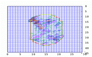
The ‘stadium billiard’ system depicted in Figure 1 is a system that is considered to be classically chaotic1 – its trajectory is very sensitive to the initial conditions and, in general, the same orbit will never be exactly retraced. The stadium consists of two semi-circular caps which, for the purposes of this study, have a diameter equal to the side length of the straight sections. This potential well was created as a step function with a quite high potential outside, thus making the walls quite ‘solid’ in a classical sense.
Another system with similar properties that is of computational interest is the ‘lemon billiard’ system depicted in Figure 2. This system has a number of quasi-periodic trajectories when treated classically, over short time spans (a few dozen orbits), however a more description of the motion indicates that in general the orbits will never be retraced.
The practical application of these systems may be seen in diffusion related problems where, for example, a solute particle may be surrounded by solvent particles, thus preventing a reaction process. In the context of these two-dimensional potentials, this process may be considered to be confined to a surface. This example may, of course, be extended to the bulk solution by considering a three-dimensional potential. The interactions of these particles is clearly not purely classical, although it is advantageous computationally to be able to treat them in a classical manner.
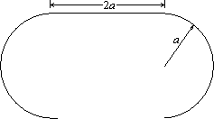
Figure 1: The ‘stadium’ billiard potential under consideration in this study.
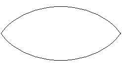
Figure 2: The ‘lemon’ billiard potential is also of interest.
Computational Investigation
Integration Techniques
The computational scheme adopted here for the solution of the Schrödinger equation is an explicit scheme in that the wavefunction at any point is calculated directly from the wavefunction in the previous time step without the need to solve simultaneous equations. The use of an Euler method in this situation is, unfortunately, not possible as it can be shown2 that for the Schrödinger equation, the Euler method is unstable. However, an explicit scheme presents significant computational advantages over the inversion of large matrices every time-step as is required in implicit schemes such as the Crank-Nicholson method. The method uses a second order difference equation and may be derived using a Taylor expansion of the implicit Crank-Nicholson method2 described as follows:
where
 ,
,Dxl are the grid size, Dt is the time step and V is the potential. Each of the functions involved has been written in discrete notation, recognising the implementation of this method. The subscripts (j,k) indicate the spatial position, whilst the superscript n indicates the time step.
In the context of the computational calculations this scheme is best viewed once split into its real and imaginary parts. Thus taking y(x, y, t) = R(x, y, t) + iI(x, y, t), where R and I are real valued functions and simplifying for the square grid used in this study yields:
![]() . (3b)
. (3b)
It may also be shown2 that the accuracy of this scheme is of the same order as the Crank-Nicholson scheme, O(Dx4). Furthermore, this scheme is stable according to the Courant-Levi-Fredrichs criterion regarding error propagation. Unlike the Crank-Nicholson implicit scheme, this method does not strictly maintain unitary probability throughout the course of the calculations. It has been established, however, that the probability remains constant to O(Dt4) (i.e. O(Dx8) for a=O(1)), which is a quite acceptable result.
It must, however, be noted that the eigenvalues of the wavefunctions that are being propagated using this explicit method are not found during the propagation process as was the case for the Crank-Nicholson method. This has serious implications for the study of systems in the semi-classical limit, as the behaviour of a system is effected quite markedly by the proximity of an eigenstate and semi-classical techniques often rely on knowledge of the eigenvalues. Further investigation of a means of determining the eigenstates present within the wavefunction is, however, outside the scope of this study.
It should also be noted that higher dimensional analogues of the method presented here may not be easily generalised from Equation 1. Rather, recourse to the general, multi-dimensional derivation is required. Furthermore, it has been noted that the source code provided with some texts purporting to use this method have not, in fact, performed this generalisation correctly (c.f. harmos.f provided by Ref. 3).
Numerical Simulations
For the purposes of this investigation, computations for this explicit scheme were performed using Fortran 90 (MIPSpro F90 compiler) on an SGI O2 with MIPS R5K processor. The algorithm was constructed so that a snapshot of the probability function, |y|2, was written out at a user-defined frequency in a format that could be viewed using the Free Software Foundation’s graphics tool gnuplot. In the numerical experiments performed, data was collected every 10 time steps, and the data was only saved on a 30×45 course grid (since saving the entire space was not required for the visualisation). Sequences of these 3D plots (two spatial dimensions plus the probability density function) were also chained together using gnuplot to provide a convenient method of observing the evolution of the wavefunction. Contour plots of the wavefunction generated by gnuplot were also used to study the wavefunction. Appendix B contains more information for optimising the performance of gnuplot for these animations.
Initially, the stability and accuracy of the algorithm were investigated by studying the wavefunction for well-known potential functions such as a ramp, flat potential and single slit. It was found that the numerical solutions maintained (at least qualitatively) symmetry, momentum and probability as required for each of these examples. Since the algorithm has been shown to be highly accurate, it was felt that it was outside the scope of this study to computationally verify the accuracy of the algorithm through comparison with the Crank-Nicholson method.
As previously mentioned, the eigenstates of the potential under consideration was not known, so it was convenient to excite a number of modes within the potential by using a Gaussian distribution as the t = 0 wavefunction. This is in some ways a representation of a localised particle at t = 0 and so although the resulting wavefunction is undoubtedly more complicated as a result, it is also more realistic and more interesting to study. A variety of initial positions and initial momenta were used to study the behaviour under different initial conditions. Of particular interest were the simulations that had a high degree of symmetry in their initial conditions as they showed some interesting properties of the system.
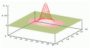
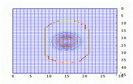
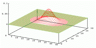
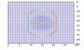
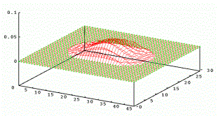
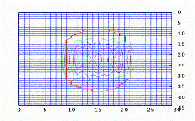
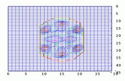
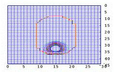
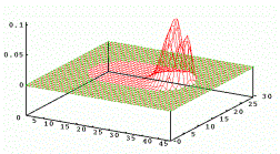
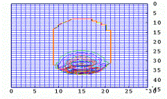
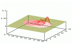
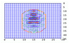
The totally symmetric mode where there is no initial momentum and the wavefunction is centred about the middle of the stadium provided an interesting insight into the semi-classical limit. A series of frames at progressive times are shown in Figure 3. It is seen in this case, that a pseudo-standing wave is generated across the stadium after a short time interval, but that the effects of the circular caps cause the mode to become more complicated, finally settling into a mode shown in Figure 3i that reflects the symmetry of the stadium.
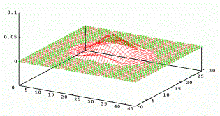
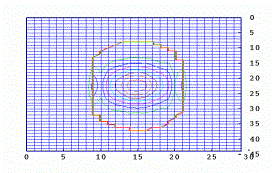
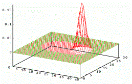
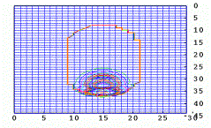
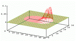
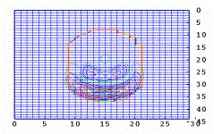
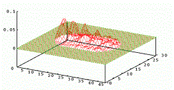
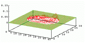
Similar patterns are observed in the wavefunction when the Gaussian is placed over the centre of the semi-circular caps. In this case, the predominant mode that is seen consists of a number of lobes down the centre of the stadium. This situation is shown in Figure 4, in both 3D plots and contour plots. In each of these experiments, the Dx = 0.2 and Dt = 0.01.
(a) (e)
(b) (f)
(c) (g)
(d) (h)
(i)
Figure 3: (a)-(d) 3D plots of the probability density function at time t = 150, 200, 250, 300 and their corresponding contour plots (e)-(h). Contour plot (i) is the mode which appears to be stable at large time (t = 1500). The stadium is coloured in to provide clarity. Note that an ‘undocumented feature’ in gnuplot is the source of the square protrusions from the stadium.
(a) (f)
(b) (g)
(c) (h)
(d) (i)
(e) (j)
Figure 4: (a)-(d) 3D plots of the probability density function at time t = 110, 150, 190, 400 and their corresponding contour plots (f)-(i). Plots (e) and (j) show the mode that becomes apparent at large time (t = 1800). See Figure 3 for more details.
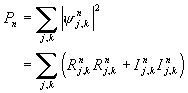
It should be noted that the total probability is given by:
for a wavefunction in a continuous space, where dt is an infinitessimal of space. In a discrete space such as the one considered here, the total probability is given by:
The plot of the total probability function for the experiment depicted in Figure 4 is shown in Figure 5 and is typical of the probability density functions generated by experiments that had no initial momentum. It may be noted that the probability is conserved to around 0.2%, and that the major deviation from unitary probability occurs when the wave packet first hits the walls of the stadium.
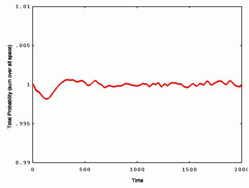
Figure 5: The total probability density as a
function of time for the experiment described in
Figure 4 - Gaussian over centre of end cap, no initial momentum.
Other numerical experiments conducted provided an initial momentum to the wavepacket. One such experiment is illustrated in part in Figure 6, starting the Gaussian from the centre of the stadium with equal momentum in x and y directions (so the wavepacket would hit the junction of the caps and the sides of the stadium). It may be seen from close inspection of this time frame (and indeed the complete sequence of frames) that there is a strong classical behaviour in this case. In Figure 6b the wavepacket is propagating top-left to bottom-right and proceeds to reflect from the walls in a classical fashion.
(a) (b)
Figure 6: One time frame (t = 1000) from a mode with initial momentum towards the join between the end caps and the sides of the stadium.
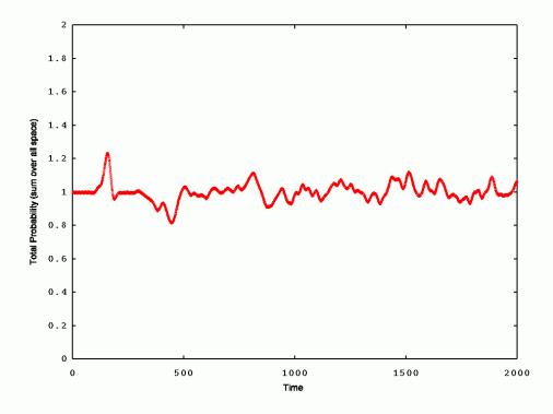
Figure 7: The total probability density as a
function of time for the experiment described in
Figure 6 - Gaussian at centre of stadium, initial momentum equal in x and y.
It may also be seen from Figure 7 that the conservation of the total probability is not nearly as rigorous as was seen for the previous experiments. Indeed, fluctuations in total probability of around 25% are observed when the wavepacket interacts with the wall of the stadium.
Discussion
The numerical experiments performed during the course of this study raise a number of interesting issues regarding the nature and accuracy of these simulations, as well as the behaviour of mesoscopic systems in the semi-classical limit. It is useful to consider the computational and semi-classical issues separately, starting with the computational points so that computational artifacts may be removed from subsequent discussion.
Probability Conservation and Algorithm Stability
As seen in Figures 5 and 7, the conservation of total probability within the explicit scheme used here is quite good in some cases (notably where no initial momentum), however, it proves to be quite poor in other situations. Since the derivation of the algorithm indicate that the probability should be conserved to O(Dt4), the natural approach is to try a smaller step size. Unfortunately, this approach does not yield the desired results. Another approach that may be investigated is a more well-behaved potential, thus testing the case that the discontinuity in the potential function at the walls of the stadium causes the probability variation. It is also possible that a better expression can be found for the probability that, perhaps, makes use of the values of the wavefunction at previous time-steps, or at neighbouring grid points. This is an area that requires a large amount of theoretical work to allow this computational scheme to be more widely applied.
Also of particular interest was the interaction between Dt, Dx and V in terms of the stability of the solution. It was found that for large Dt, small Dx, or large V the wavefunction became infinite after only a few time-steps. This may be a function of the limited precision of the numeric computations, or the discrete nature of time and space in these simulations. Once again, more theoretical work is required to allow this potential problem to be overcome.
Semi-classical consequences
It has been seen in this study that with some modes of excitation, this system behaves in a very wave-like manner (particularly the totally symmetric mode in Figure 3). The modes observed in these situations are such that, in general, this system cannot be described adequately by classical mechanics. Careful analysis of the data provided by the experiment described in Figure 6, however, indicates that in many cases, a classical treatment of the situation may be possible (and hence desirable). This tendency for the quantum mechanical solution to provide very similar answers to the classical solution in some stadia has been described as ‘scarring’ of the wavefunction1 and provides the basis on which semi-classical methods may be built.
Conclusions
It has been seen from the numerical experiments performed here that there are many unresolved issues surrounding this current area of research – in particular the performance of this explicit integration scheme. The most pressing problem is currently the conservation of total probability within the system. In addition to that, it would be desirable to calculate the total energy of the system and check to see that it too, is conserved. It should, of course, be noted that the calculation of the kinetic energy in this explicit scheme presents significant computational challenges that must be overcome. There is also scope for further research involving different dimensions for the stadium and other interesting shapes such as the ‘lemon’ billiard system. To fully appreciate the significance of these results, more rigorous comparison to the classical results is also required, including (but not limited to) the calculation of classical trajectories and the preparation of correlation functions for the classical and quantum solutions.
It can, however, be concluded directly from this study that the stadium billiard system provides many challenges both computationally and theoretically that must be overcome before semi-classical methods can become widely used. It has been shown in the numerical experiments performed here that this system can behave quite classically, or quite quantum-mechanically depending on the initial conditions. This makes the stadium billiard system ideal for further semi-classical studies.
Acknowledgments
My thanks go to A/Prof. Bernard Palethorpe and Mr Daniel Mitchell for their assistance in this computational work and Dr Nicole Bordes for her assistance in data visualisation. Also thanks to Dr Peter Harrowell (School of Chemistry) for providing the inspiration for this study.
The results were generated using the Sydney Regional Visualisation Laboratory which is supported by the Australian Research Council.
References
1. Heller E.J., and Tomsovic S., Physics Today July 1993.
2. Askar A. and Cakmak A.S., J. Chem. Phys. 68, 2794 (1977).
3. Landau R.H. and Páez M.J., Computational Physics: Problem Solving with Computers, John Wiley & Sons, 1997.